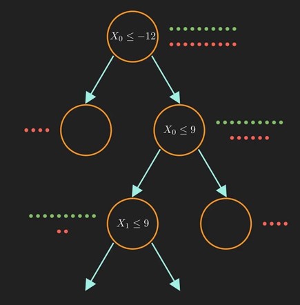
Decision trees are a collection of yes/no questions organized in a tree structure for classification. Each yes/no question is called a node. By convention: - YES leads to the left child. - NO leads to the right child.
At each node, the dataset is split into two subsets, and the process recurses as shown in the figure below.
Decision trees can be used for regression and classification, hence, some people call them Classification And Regression Trees (CART).
How to Fit a Decision Tree
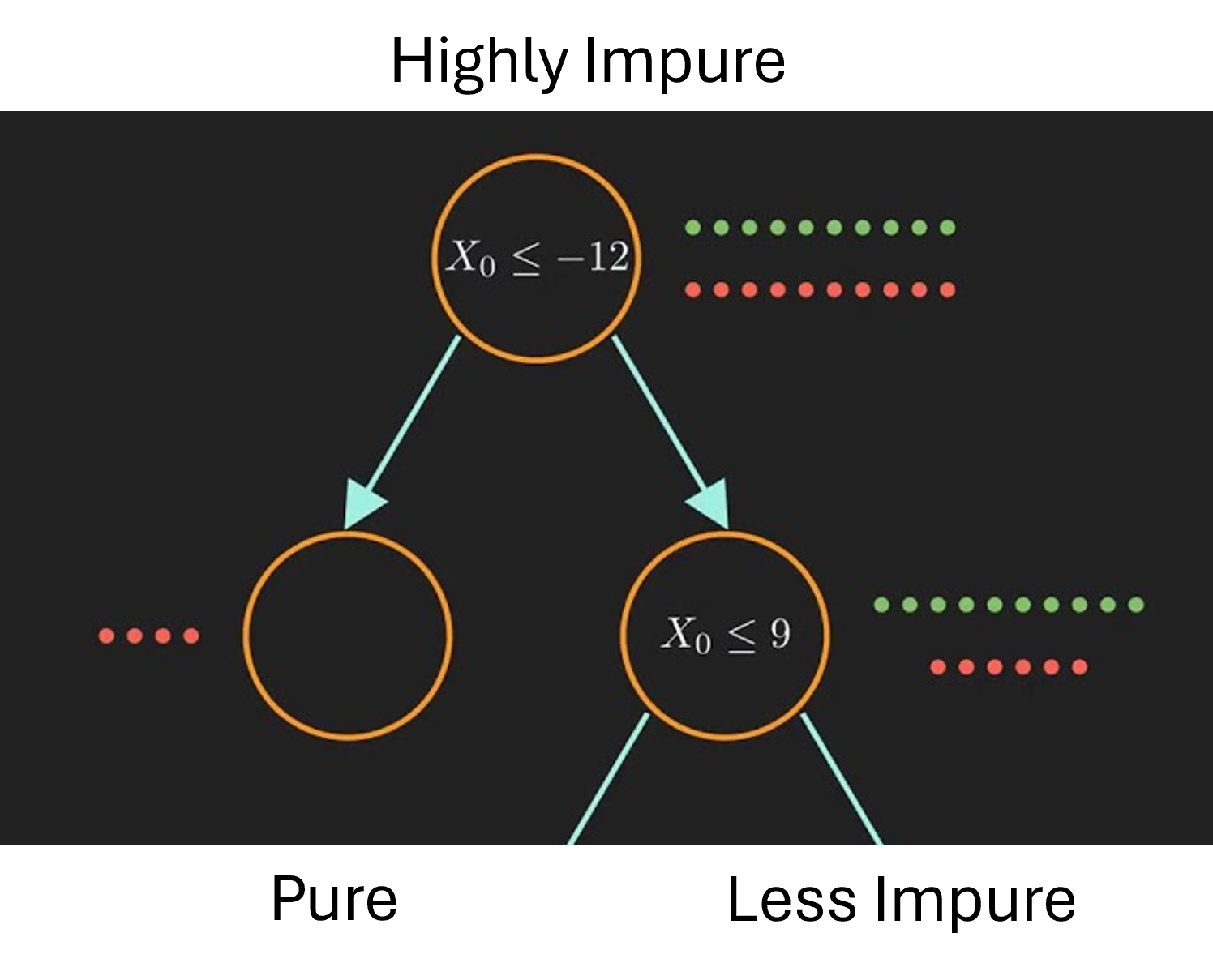
Each node has a greedy target: Minimize the impurity of both child nodes, in other words to lower the diversity of each node. This can be achieved by:
Reducing the number of unique classes of each child node.
Making the distribution of classes less even.
A pure node is such nodes that contains observations of a single class, signaling the end of recursion. The following image shows different levels of impurity
Measuring Impurity
Gini Index
The Gini index measures node impurity by evaluating the probability of incorrect classification. Mathematically, it is the probability that two randomly selected observations from the node belong to different classes. Note: \(P(different) = 1 - P(same)\)
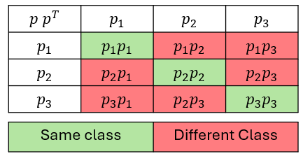
Observe that if \(p\) is the vector containing the class proportions for a node, then \(p\,p^T\) gives computes a matrix representing the entire sample space of class combinations.
We can observe that \(P(same) = \operatorname{trace}(p\,p^T) = p \cdot p\). Thus, the Gini index can be written as:
\[
\text{Gini Index}(p) = P(different) = 1- P(same) = 1 - p \cdot p = 1 - \sum_{i=1}^k p_i^2
\]
While the dot product is sufficient to express the Gini index, it most comonly found using the sum notation at the end of the expresion
Entropy
Entropy is also used to measure diversity in the context of biology and ecolofy, often referred to as the Shannon Diversity Index. It was originally derived for information theory where by using \(\log_2\) it represents the expected number of questions needed to reach a pure node. In practice, for decicion trees, entropy is normalized to [0,1] using \(\log_k\) for interpretability and comparability with the Gini index.
However, Information Gain is preferred over entropy in practical applications. Both the GINI Index and Entropy give us absolute measures, but in the context of decision trees, we have a previous state we’d like to compare against. Information gain is a relative measure that achieves this. Information Gain is analogous to “Lost Surprise”. Since Entropy is also analogous to surprise, the formula is as follows:
To select the best question, we first need to consider which questions to ask. This changes between continuous and categorical variables. Once we have a list of questions, we can evaluate them using the above formula. And select the question that maximizes information gain or minimizes the gini coefficient.
Height
Weight
Gender
School Year
Likes Pokemon?
165
55
Female
Sophomore
Yes
178
72
Male
Junior
No
160
50
Female
Freshman
Yes
172
65
Male
Senior
Yes
155
48
Female
Sophomore
No
168
60
Male
Freshman
Yes
For Continuous Variables
To identify the best question for continuous variables, we need to consider smart cut-off points. To avoid asking redundant questions, the following steps can be used: 1. Sort the data. 2. Evaluate potential questions at in-between values (or percentiles for larger datasets). 3. Measure the “goodness” of each question. 4. Choose the best one.
Example with heights:
Sorted Data:
Height
Likes Pokemon?
155
No
160
Yes
165
Yes
168
Yes
172
Yes
178
No
Questions:
Q1: Height ≤ 157.5?
Q2: Height ≤ 162.5?
Q3: Height ≤ 166.5?
Q4: Height ≤ 170.0?
Q5: Height ≤ 175.0?
Then, we’d compute the relevant metric for each of the questions and choose the best one.
For Categorical Variables
For categorical variables, it is a little bit easier. We can just ask if the value is in a certain category or not. Then we measure how good each question is and choose the best one.
Example with School Year
Sorted Data:
School Year
Likes Pokemon?
Sophomore
Yes
Junior
No
Freshman
Yes
Senior
Yes
Sophomore
No
Freshman
Yes
Questions:
Q1: Is Sophomore?
Q2: Is Junior?
Q3: Is Freshman?
Q4: Is Senior?
Recursive Fitting of a decision tree.
Now that we understand all the components needed to fit a decision tree, let’s see how we can fit a decision tree recursively:
Indentify the best question for each variable.
Indentify the best question among all variables.
Use that question to split the data into child nodes.
Recursively apply the process to child nodes.
Stop when the data is pure or the tree is too deep*.
Prediction Using a Tree
To make predictions, traverse the tree by answering the yes/no questions until reaching a leaf node. Then, if we’re classifying use the majority class of the leaf node, if we’re regression use the mean of the leaf node.
Impurity for regression
While we discussed impurity before, it was focused on clasiffication. For regression, we use the variance of the target variable for that specific node.
Pros and Cons of Decision Trees
Pros
Computationally efficient.
Highly interpretable.
Captures non-linear relationships.
Automatically detects feature importance.
Fast training and prediction.
Handles both numerical and categorical data.
Cons
Prone to overfitting.
Sensitive to data variability.
Biased toward dominant features.
Greedy algorithm arrow Less accurate on test sets.
Overcoming Overfitting
Regularization parameters include: - Max depth: Limit the tree’s depth. - Min samples split: Minimum number of samples to split a node. - Min samples leaf: Minimum samples in a leaf node. - Min impurity decrease: Minimum decrease in impurity to split further. - Pruning: Remove leaf nodes that minimally reduce impurity.
Addressing Limitations with Ensembles
Ensemble models enhance decision tree performance: - Random Forest - AdaBoost - GradientBoost - XGBoost
While algorithms like AdaBoost and GradientBoost are general ensemble methods, they are widely associated with tree-based models.
Not PyTorch
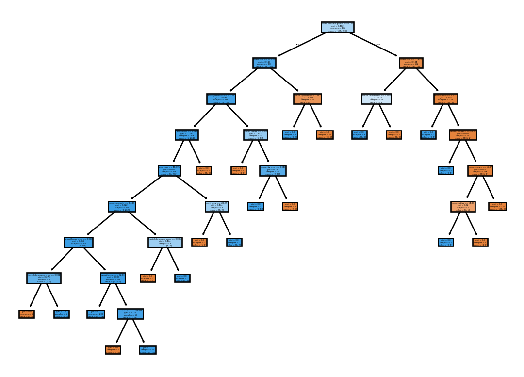
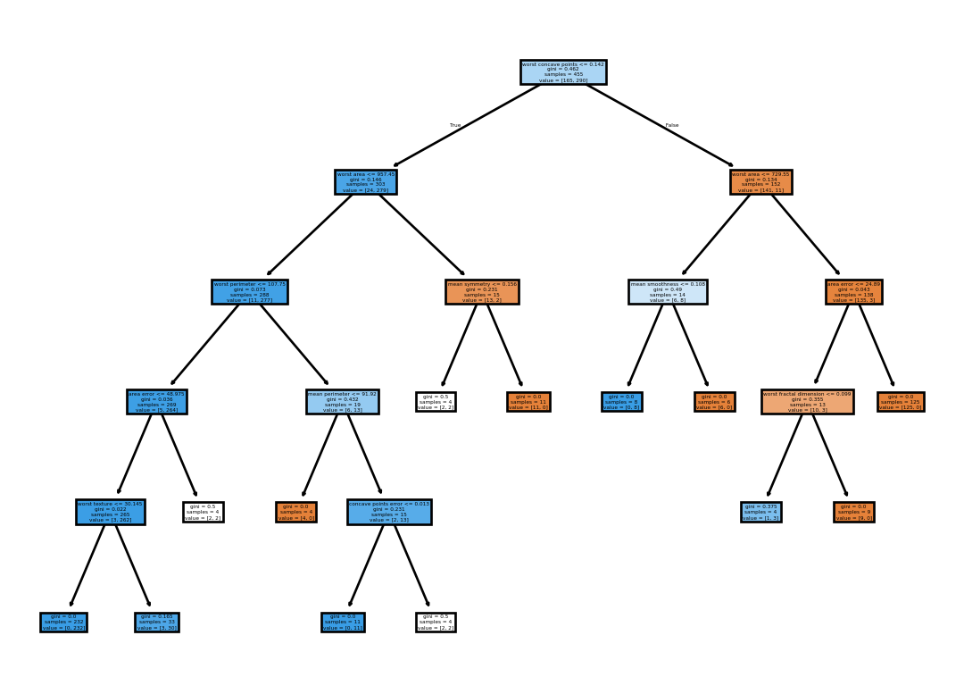
The SciKit-Learn library in Python provides a comprehensive implementation of decision trees. For this showcase we’ll fit a classification tree to the breast cancer dataset.
Blue nodes represent observations that are classified as benign, while orange nodes represent observations that are classified as malignant. The more intense a node is colored, the purer it is. However, the tree is so large that it is difficult to interpret. It is also very likely that it is overfit. So,let’s take a look at the train and test accuracies:
Yup, the train accuracy is 100% and the test accuracy is 91%. This is a classic example of overfitting. Let’s fit another tree with some regularization parameters and analyze the results.
The Train accuracy decreases to 97%, but the test accuracy jumps all the way to 96%. This is a good example of how regularization can help prevent overfitting.
However, I must admit I originally didn’t set any seeds, which gave varying results each time I ran the code (mostly due to the train/test split). Different seeds gave widely different results, which is not ideal. The test accuracies in both cases ranged between 88%-95%, showing that trees are very sensitive to changes in the data.
This is a high-level summary of decision trees, offering insights into their structure, fitting process, and how to improve their performance using regularization and ensemble methods.