Convolutional Neural Networks

As we discussed previously, Multi-layer Perceptrons (MLP) are not very good at image classification. This is because they do not take into account the spatial relationships between pixels. In this chapter, we will discuss Convolutional Neural Networks (CNNs), which are specifically designed to handle image data.

Convolution

Before we discuss CNNs, we need to understand the concept of convolution. Convolution is a mathematical operation that is used takes in an input vector, \(f\), and a kernel vector, \(k\), and performs a sliding window weighted sum of \(f\), with \(k\) acting as weights. Each weighted sum can be represented by a dot product. The convolution operation is defined as follows: \[ (k * f)[i] = \sum_{j=0}^{m-1} k[j] f[i+j] \]

for \(i \in \{0, \ldots, n-m\}\).

Where \(k\), the kernel, is an \(m\)-vector and \(f\), the input is and \(n\)-vector. The result of the convolution is a vector of length \(n-m+1\). Note that we’re using brackets notation (\([]\)) instead of subindeces, as we go deeper this notation is clearer as we introduce more indices.

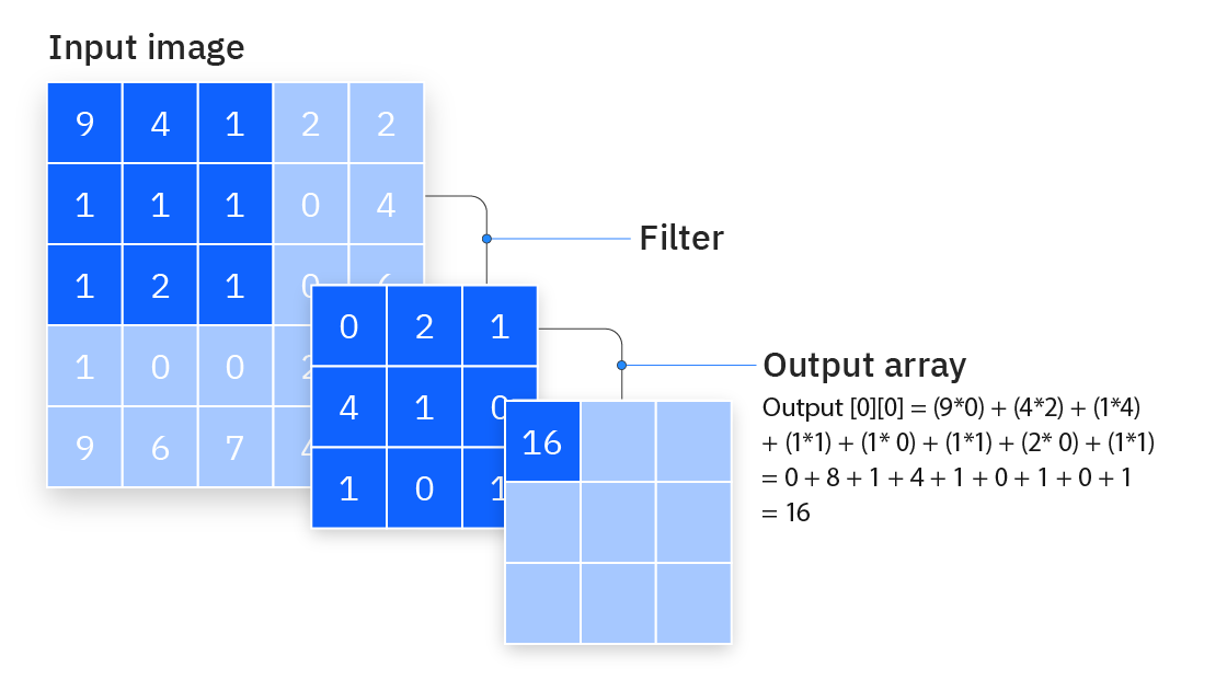
This concept can be expanded into a 2D case using the following formula:

\[ (k * f)[i_1, i_2] = \sum_{j_1, j_2=0}^{m-1} k[j_1, j_2] f[i_1 + j_1, i_2 + j_2] \]

for \(i_1 \in \{0, \ldots, h-m\}\) and \(i_2 \in \{0, \ldots, w-m\}\).

Where \(k\), the kernel, is an \(m\times m\) matrix and \(f\), the input is an \(h\times w\) matrix representing an image. The result of the convolution is a \((h-m+1) \times (w-m+1)\) matrix.

The 2d Convolution is also a sort of sliding window weighted sum operation as depicted by the following figure:

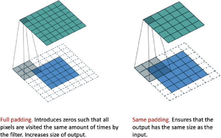
Padding

The previous image shows that a convolution operation reduces the size of the input image. This is not always desirable, especially when the image is small. To avoid this, we can pad the input image with zeros. There are three main padding types: none or valid, same, and full. The first one represents no padding, the second one represents padding such that the output has the same size as the input and the last one represents padding such that the output uses all the possible information. These are not the only types of padding, we can also give an arbitrarily sized padding. The following figure shows the effect of padding on a 2D convolution:

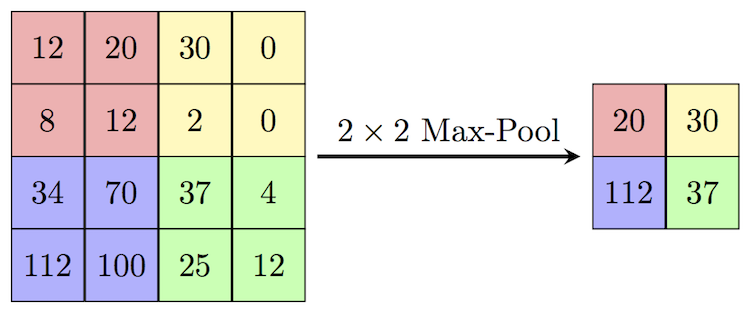
Max Pooling

Max pooling is a downsampling operation that reduces the size of the input tensor. It is a sliding window operation that takes the maximum value of the window. In the context of CNN’s it acts as an activation function. There are two main parameters for max pooling: the window size and the stride. The window size is the size of the sliding window and the stride is the number of steps the window takes in each direction. The following figure shows the effect of max pooling on a 2D tensor:

Convolutional Layers and Networks

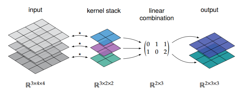
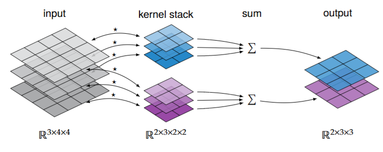
An image isn’t just a 2D matrix/tensor, specially if it has multiple color channels (e.g. RGB). As such, we need a 3-tensor to represent an image with several channels. It is tempting to define the shape of the 3-tensor as \(h \times w \times c\) where \(c\) is the number of color channels, however, for reasons that will become aparent soon, it’s better to define it as a \(c \times h \times w\) 3-tensor. This way we can interpret our tensor as a stack of \(c\) 2D matrices, each of shape \(h \times w\) representing one of the channels.

Each of these channels represents a different feature of the image. As such a convolutional layer will take in \(c_\text{in}\) channels and output \(c_\text{out}\) channels. Thus, the output will have shape \(c_\text{out} \times h \times w\). There are two main ways to implement a convolutional layer

Single-channel convolution: Each input channel is convolved with a different filter, then a linear transformation to these convolutions produces the output channels.

Multi-channel convolution: Each input and output channel have their own filter, then all the convolutions corresponding to each output channel are summed together to produce the output channels.

In the end our goal is to learn the components of the kernels. Mathematically, one can be obtained from the other, so single-channel convolution is often used in practice as it has less free parameters.

Finally, it is good practice to use convolution layers followed by MaxPool layers to reduce the spatial dimensions of the output. Then, flatten the output and feed it into a (series of) fully connected layer. The follwing picture shows a schematic for a CNN:

PyTorch

Previously, we showed that a MLP struggled to classify MNIST digits. Let’s see if a CNN can do better. To avoid walls of code, most of it has been folded by default. You can unfold it by clicking the arrow in the top right corner of the code block.

Libraries and data

import torch
import torch.nn as nn
import torch.nn.functional as F
import torchvision
import torchvision.transforms as transforms
import os
from tqdm import trange

device = torch.device("cuda" if torch.cuda.is_available() else "cpu")

# Load and normalize the training and test sets
transform = transforms.Compose([
    transforms.RandomHorizontalFlip(p=0.5),
    transforms.RandomRotation(10),
    transforms.ToTensor(), 
    transforms.Normalize((0.5,), (0.5,)),
])

# Load the MNIST dataset
trainset = torchvision.datasets.MNIST(
    root='./data', 
    train=True, # training set
    download=True, 
    transform=transform
)
testset = torchvision.datasets.MNIST(
    root='./data', 
    train=False, # testing set
    download=True, 
    transform=transform
)

We’ll be using the following model:

class ConvolutionalMNISTClassifier(nn.Module):
    def __init__(self):
        super(ConvolutionalMNISTClassifier, self).__init__()
        self.layers = nn.Sequential(
            nn.Conv2d(1, 4, kernel_size=3, padding=1),
            nn.ReLU(),
            nn.Conv2d(4, 8, kernel_size=3, padding=1),
            nn.ReLU(),
            nn.MaxPool2d(kernel_size=2, stride=2),
            nn.Conv2d(8, 8, kernel_size=5, padding=1),
            nn.ReLU(),
            nn.Conv2d(8, 8, kernel_size=5, padding=1),
            nn.ReLU(),
            nn.MaxPool2d(kernel_size=2, stride=2),
            nn.Flatten(),
            nn.Linear(200, 64),
            nn.ReLU(),
            nn.Linear(64, 10),
        )

    def forward(self, x):
        return self.layers(x)

Training the model

# hyperparameters
batch_size = 64
num_epochs = 5
learning_rate = 0.001

# Create the model
model = ConvolutionalMNISTClassifier().to(device)

# Define the loss function and the optimizer
criterion = nn.CrossEntropyLoss()
optimizer = torch.optim.Adam(model.parameters(), lr=learning_rate)

# Train the model
trainloader = torch.utils.data.DataLoader(trainset, batch_size=batch_size, shuffle=True)

if os.path.exists("models/cnn_mnist_classifier.pth"):
    state_dict = torch.load("models/cnn_mnist_classifier.pth", weights_only=False)
    model.load_state_dict(state_dict)

else:
    # Train the model
    model.train()
    for epoch in trange(num_epochs):
        for images, labels in trainloader:
            images = images.to(device)
            labels = labels.to(device)

            # Forward pass
            outputs = model(images)
            loss = criterion(outputs, labels)

            # Backward and optimize
            optimizer.zero_grad()
            loss.backward()
            optimizer.step()

    # save model
    torch.save(model.state_dict(), "models/cnn_mnist_classifier.pth")

Testing the model

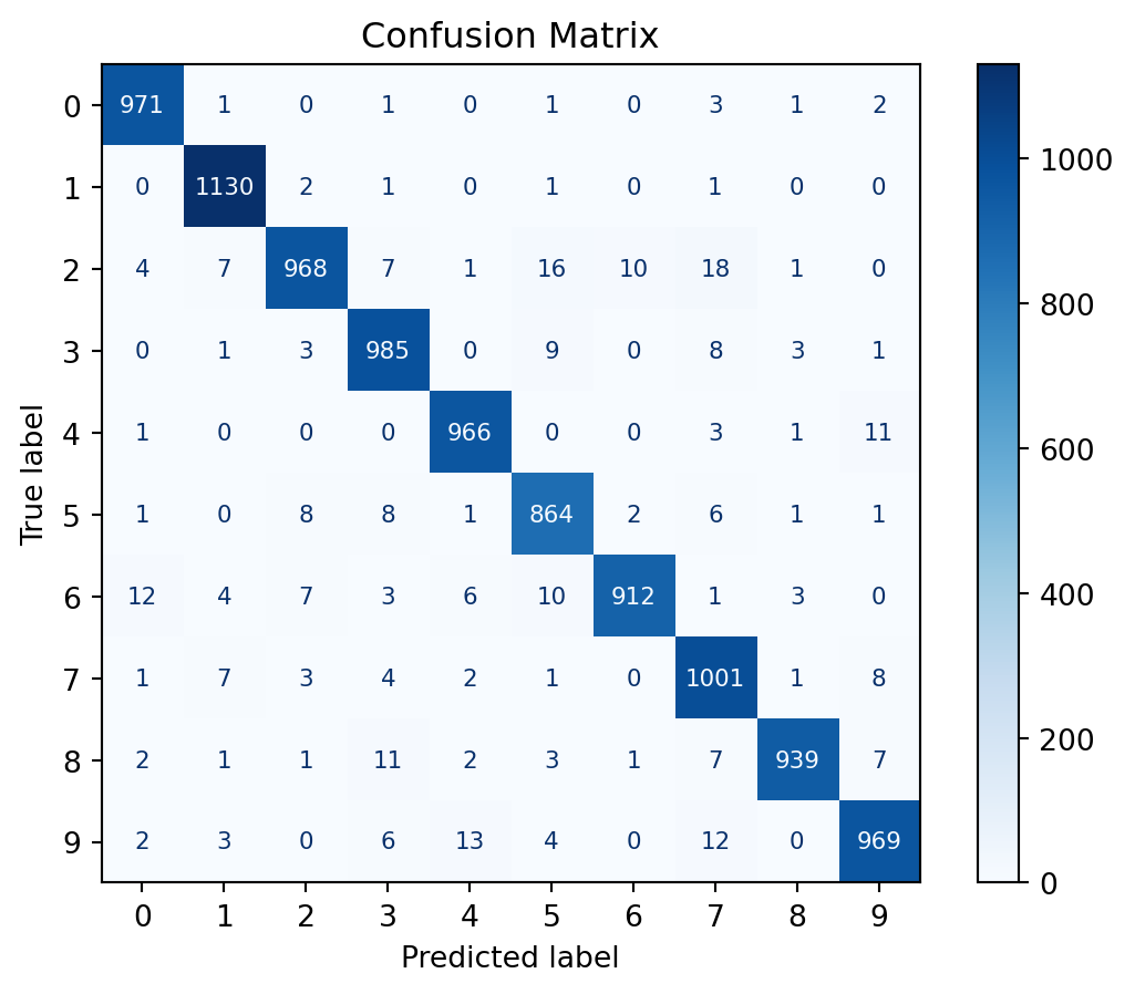
import matplotlib.pyplot as plt
from sklearn.metrics import accuracy_score, confusion_matrix, ConfusionMatrixDisplay

# retrieve data in sklearn format
X_test = torch.stack(list(zip(*testset))[0]) # exhaust the iterator, unzip, get xs, stack
y_test = testset.targets

# set model to evaluation mode
model.to("cpu")
model.eval()

# test
with torch.no_grad():
    # argmax returns the index with the highest probability, the predicted class
    y_pred = model(X_test).argmax(dim=1)

# compute confusion matrix
cm = confusion_matrix(y_test, y_pred)
disp = ConfusionMatrixDisplay(confusion_matrix=cm)
disp.plot(cmap=plt.cm.Blues, 
          text_kw={'fontsize': 8, 'ha': 'center', 'va': 'center'})

# Format numbers as integers without scientific notation
for text in disp.text_.ravel():
    text.set_text(f'{int(float(text.get_text()))}')

plt.title('Confusion Matrix')
plt.show()

# compute accuracy
accuracy = accuracy_score(y_test, y_pred)
print(f"Accuracy: {accuracy}")

Accuracy: 0.9705

As we can observe, we get an almost perfect test accuracy of 97% with a model using just under 10k parameters. Meanwhile the MLP classifier achieved 16% test accuracy with almost 40k parameters. This shows that Convolutional Neural Networks are much more powerful than Multi-Layer Perceptrons for image classification tasks.